Introduction
This posting demonstrates, from start to finish, the process of:
Preparation
This posting has presented the step-by-step process for creating, configuring and publishing an Excel 2010 workbook to SharePoint's Excel Service in order to make it generally available to other users. The external connection used by this workbook is embedded in the workbook itself. By working through this posting, one gains experience in how to configure an Excel workbook to connect to external data and in how to publish a workbook to SharePoint. For additional detail on any of the topics discussed in this posting, pleased consult the references below.
References
This posting demonstrates, from start to finish, the process of:
- Creating an Excel workbook that connects to external data using Windows authentication;
- Modifying the external data connection to focus on specific data;
- Configuring the PivotTable;
- Configuring a PivotChart; and
- Publishing the workbook to SharePoint Server 2010 Excel Services.
Preparation
- Add a blank site to the target web application, naming it AdventureWorks:

- Configure the site to inherit global navigation from the parent:

- Add a document library to this site, naming it Workbooks:

- Restore the database, AdventureWorks2008R2Full Database Backup to a SQL Server instance hosted within the same domain as the SharePoint Server 2010 farm:


- Launch Excel 2010 on a workstation hosted within the same domain as the target SharePoint Server 2010 farm, naming the new workbook SalesOrderHeader.
- On the Data ribbon, go: Go External Data > From Other Sources > From Data Connection Wizard:This opens the Data Connection Wizard.

- Select Microsoft SQL Server:

- Click Next. Enter the name of the SQL Server Database instance hosting the AdventureWorks database, and then select Windows Authentication:

- Click Next. From the dropdown, select the table, SalesOrderHeader:It's located towards the bottom of this listing. This listing cannot be sorted.

- Click Next. Enter values for File Name, Friendly Name and Search Keywords; and leave the checkbox unchecked:Leaving the checkbox unchecked causes the data connection to be embedded in the Excel file itself. Checking this option causes the connection data to be stored in and used from an external data connection (odc) file.

- Click the Authentication Settings button. Ensure that Windows Authentication has been selected:

- Click OK. The Excel Services Authentication Settings dialog closes.
- Click Finish. The Data Connection Wizard dialog closes, the Import Data dialog appears:

- Select PivotTable Report. Only pivot tables can be refreshed on the SharePoint Server, once published and viewed by a user.
- Click OK. The Import Data dialog closes, and the spreadsheet is populated with the data from the AdventureWorks table:

- This completes this step


- On the Data ribbon, look for the Connections button:

- Click Connections. The Workbook Connections dialog appears:

- Click the Properties button. The Connection Properties dialog appears:

- Select the Definition tab.
- From the Command type dropdown, select SQL.
- In the Command text box, delete the contents, and replace with the following:The Definition tab will then look like this:


- Click the Authentication Settings button. The Excel Services Authentication Settings dialog appears.
- Select Windows Authentication:
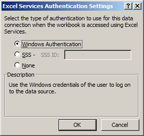
- Click OK. The Excel Services Authentication Settings dialog closes.
- Click where it states, Click here to see where the selected connections are used. This updates what is displayed in the bottom panel with the workbook location of the data obtained from the external data connection:

- Click Close. The Excel workbook sheet pivot table updates and now displays fewer fields in the PivotTable Field List panel:
- This completes this step 2.


- Drag-and-drop the fields, in the Pivot Field List, as shown:

- On the Design ribbon, click Report Layouts and then point to Show in Tabular Form:

- Click this option. The pivot table updates to display the data in tabular form:

- On the Options ribbon, in the Show section, click the +/- button. The pivot table updates and no longer displays the show/hide (+/-) button.
- On the Design ribbon, click Report Layout, and then select Repeat All Item Labels. The spreadsheet updates to repeat the labels shown in the CountryCode column.
- On the Design ribbon, click Subtotals, and then point to Do Not Show Subtotals:

- Select this option. The pivot table updates and no longer shows subtotals:

- At the top of the column to the immediate right of the Sum of TotalSales column, enter the column header SelectedCurrencyValue:

- Click once anywhere in the columns at left, to bring back the Pivotable Field List panel, and then click the small dropdown on the OrderDate button, which brings up a popup menu:

- Select Move Up. The PivotTable updates to now display the OrderDate column first:

- In the field just below the new SelectedCurrencyValue header, enter the following:
=GETPIVOTDATA("TotalSales", $A$1, "OrderDate", A2, "Territory", C2, "CountryCode", B2)*ExchangeRate - The order of the field names in this function is critical. They must be exactly in the same order as the columns in the PivotTable.
- Press Enter. The cell updates to display the function value:

- Scroll down to the bottom of the PivotTable and note down the row number for the last row of data. For this posting, the row number is: 5832. Then scroll back to the top.
- In the Name field, enter E2:E5832. This causes the enter column to be selected (except for the header).
- Press CTRL+D. This causes the function in E2 to be repeated for all of the other cells in this column:

- In the Name field, enter A1:E5832, and then press Enter. This causes all of the data rows and the header row to be selected:

- In the Name field, overwrite any value there with the value SourceDataTable, and then press Enter. This assigns a name to all that was selected, effectively creating a source of data:

- Select Sheet2.
- In cells A1 and B1 enter these values:
- Exchange Rate.
- 1.
- Select cell A2, and then in the Name field (currently displaying A2), overwrite this with ExchangeRate:This assigns that cell a variable name.

- In cell A2 and B2, enter these values:
- Currency Code.
- USD.
- Select cell B2, and then in the Name field (currently displaying B2), overwrite this with CurrencyCode:

- In cell A3 and C3, enter these values:
- Chart Title.
- ="Sales in " & CurrencyCode.
- Select cell C3, and then in the Name field (currently display C3), overwrite this with ChartTitle:

- To review all of the cell and table variables that have been created thus far, on the Formulas ribbon, in the Defined Names section, click Name Manager. The Name Manager dialog appears:

- This completes Step 3.


- Select Sheet3.
- On the Insert ribbon, click PivotTable. The Create PivotTable with PivotChart dialog appears:

- Enter the name for the source data table created previously, SourceDataTable, and then click OK. The sheet update to display a blank PivotTable, PivotChart and PivotTable Field List panel:
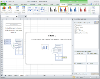
- On the PivotTable Field List panel, drag fields into the Axis Fields, Legend Fields and Values boxes like so:

- Then move the chart and resize it so that it fills the viewable area:

- Select the chart. This activates the PivotChart Tools ribbons.
- On the Layout ribbon, click Chart Title, and then point to Above Chart:

- Click this option. A title field is added to the chart, displaying a default value:

- Select the chart title field, and then enter the following into the Formula bar:
=SalesOrderHeader.xlsx!ChartTitle

- Select the chart to activate the Chart ribbons.
- On the Design ribbon, click the Change Chart Type button. The Change Chart Type dialog appears:

- Hover the cursor over the various images displayed in this dialog to view the names of the different chart types.
- Select the Stack Chart type, and then click OK. There will appear to be little noticeable difference in the chart, but this is due to the amount of data currently displayed by the chart, which tends to obscure such things.
- On the Design ribbon, in the Chart Styles section, expand the chart styles panel and then point to Style 16:

- Click on Style 16. Again, there will be little noticeable change in the chart currently displayed. However, this change will become apparent, when zooming into date ranges using the filter options. Additionally, these chart options must be set now before publishing to the SharePoint Server instance, as, once published, they cannot be changed from the web interface.
- This completes Step 4.


- On the Excel UI, select the File tab, at far left.
- On the File tab, go: Save & Send > Save to SharePoint:

- Double-click Browse for a location. The Save As panel appears.
- In the File Name field, enter the path to the document library created in step 1:

- Press Enter. After a few moments, the Save As dialog updates to display the SharePoint Server 2010 document library location.
- Enter the name of the Excel 2010 workbook, SalesOrderHeader:

- Be sure to also check: Open with Excel in the browser.
- Press Enter. A progress bar appears momentarily. Then a new browser instance is launched and connected to the web-enabled workbook displaying a warning message:

- Click Yes. After a few moments, the browser displays the web-enabled workbook:

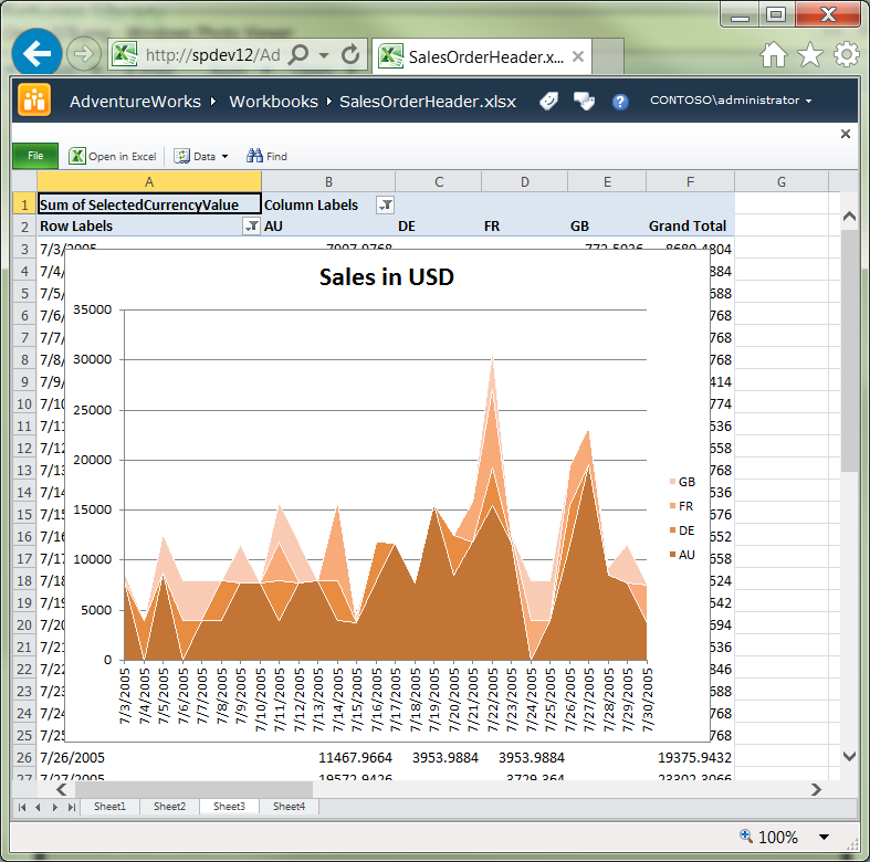
- Click the Row Labels dropdown, point to Date Filters and then point to Between:.
- Click Between. A Custom Filter dialog appears.
- Enter the between dates 7/3/2005 and 7/30/2005:

- Click OK. The chart updates to display a filtered date-range of values:

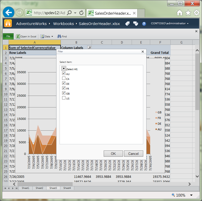
- Click the Column Labels dropdown, and then point to Filters:

- Click Filters. The Filter dialog appears.
- Uncheck the CA and US items:

- Click OK. The chart updates to display just the sales for GB, FR, DE and AU:

- This completes Step 5.


- Launch Central Administration.
- Go: Central Administration > Application Management > Manage Service Applications > Excel Services Application > Trusted File Locations:

- Click on the http:// link listed there. The Edit Trusted File Location page is displayed.
- Scroll down to the Session Management section.
- Change the Sessions Timeout and Short Session Timeout values to 20 minutes (1200 seconds):

- Click OK.


This posting has presented the step-by-step process for creating, configuring and publishing an Excel 2010 workbook to SharePoint's Excel Service in order to make it generally available to other users. The external connection used by this workbook is embedded in the workbook itself. By working through this posting, one gains experience in how to configure an Excel workbook to connect to external data and in how to publish a workbook to SharePoint. For additional detail on any of the topics discussed in this posting, pleased consult the references below.
References
- TechNet Library SharePoint 2010
- Configure Excel Services for a BI test environment
- Chapter 12: Excel Services (SharePoint 2010 Web App The Complete Reference)
- Configuring a BI infrastructure: Hands-on labs
- Configure Excel Services Application settings (Office Web Apps)
- What's new for Excel Services (SharePoint Server 2010)
- Excel Services administration (SharePoint Server 2010)
- Configure Excel Services data refresh by using the unattended service account (SharePoint Server 2010)
- Plan Excel Services authentication (SharePoint Server 2010)
- Manage Excel Services trusted locations (SharePoint Server 2010)
- Al's Tech Tips
- Microsoft Office
- Publish a workbook to a SharePoint site
- Differences between using a workbook in the browser and in Excel
- Refreshing data in a workbook in a browser window
- Refresh external data in a workbook in the browser
- Business intelligence in Excel and Excel Services (SharePoint Server)
- Sessions and session time-outs in a workbook in the browser
- Blogs
- Uncovering Publish to Excel Services in Excel 2010
- Using Office Data Connection files (.odc) and the DataConnections Web Part in SharePoint to Specify External Data Connections in Newly Created Excel Workbooks
- Excel Services delegation
- SQL Server Database product Samples
- By default, Session Timeout is 450 seconds, or 7.5 minutes. Longer session times can be configured through the Excel Services Application.
2 comments:
Hello! I know this is sort of off-topic however I had to ask.
Does operating a well-established website such as yours require a large amount of work?
I am brand new to operating a blog however I do write
in my journal daily. I'd like to start a blog so I can easily
share my experience and thoughts online. Please let me know if you have
any suggestions or tips for new aspiring blog owners.
Appreciate it!
It is a lot of work, but it's useful work. I write postings primarily for my own needs: this is my online library. I refer to it and use it constantly in my own work. I need it because there is too much to remember all the time. I have worked with tech specialists who keep such notes in a paper journal. I keep them online for ease of access. My objectives in writing a posting is to be completely objective, clear and factual; minimizing or removing all unessential comment; and presenting topics step by step, including every step no matter how trivial. This approach does require extra effort, but the effort returns value by ensuring that the posting remains useful long after it has been written.
Post a Comment