Build querystring from form field data

Here's a simple way of getting form field data from a SharePoint form, adding that data to a URL, and then causing the browser to navigate to that URL.  It assumes a form named MyForm and a textbox element named TextBox1.  Additional parameters can be added as needed. This gets you started:

function setMyFormURL()
{
  var string = document.getElementById('Textbox1').value;
  var urlString = '~/sitepages/myFile.aspx?fn=' + string;
  document.location.href = urlString;
}
.
.
.
OnClientClick='JavaScript:setMyFormURL();return false;'

References

• Button.OnClientClick Property

How to create a no-code drill-down chart in SharePoint 2010

Introduction

This posting walks you through the process of creating an out-of-the-box, no-code drill-down chart in SharePoint 2010.  It uses the Northwind sample database transformed to SharePoint 2010 for data, specifically the Products and Categories lists.  The Categories list is related to the Products list through a one-to-many relationship.  The process involves several discrete steps:

1. Inserting the Chart web part onto the target page.
2. Adding a count field to the Categories list that automatically counts the number of occurrences of a Category item in the Products list.
3. Connecting the Chart web part to the Categories list.
4. Configuring Chart drill-down capability.

Step 1: Insert the Chart web part

1. Launch SharePoint Designer 2010, and then connect to the target site.
2. In Designer insert the Chart web part onto the target page.
3. Next, in Code view, search for the ShowToolbar parameter, and then set this to False.  You will not need to go to Advanced Mode to make this change.
4. Select the Chart web part inserted on the page, and then, on the Format ribbon, click Chrome Type, and then click None.
5. Click the Chrome State button, and then click Normal.
6. Save the file and then exit Designer.
7. You should see something like the following:
   

Step 2: Add count column to Categories list

1. Launch a browser, and then connect to the target site.
2. Navigate to the Categories list:
   
3. Select the List ribbon.
4. In the Manage Views group, click the Add Column button (to find it, hover the cursor over ribbon items to view a popup title of the item).  The Create Column modal dialog appears.
5. Configure as follows:
1. Column name: Count.
2. Type of information: Lookup.
3. Get information from: Products.
4. In this column: Category (Count Related).
5. Leave all other fields default:
   
6. Click OK.  The Categories list now displays the number of times that each category was used in the Products table:
   

Step 3: Connect Chart to Categories list

1. Launch a browser and then connect to the target page.
2. On the Page ribbon, click Edit Page.
3. As you move the cursor over the chart web part, a dropdown will appear across from the web part title. Click the dropdown, and then point to Connect to Data:
   
4. Click this menu item.
5. Select Connect to a List.
6. Click Next.
7. Select the site where the Products list is hosted; select the Categories list.
8. Click Next.
9. Click Next.
10. Expand the Series Properties area, and then configure as follows:
1. Series Name: CategoryCounts.
2. Series Type: Bar.
3. Leave all other fields default:
   
11. Click Finish.

Step 4: Configure chart drill-down capability

1. NOTE: after making each change below, press ENTER.  Changes can be made only one at a time, as each change triggers a page reload.
2. Launch a browser and then connect to the target page.
3. On the Page ribbon, click Edit Page.
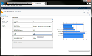
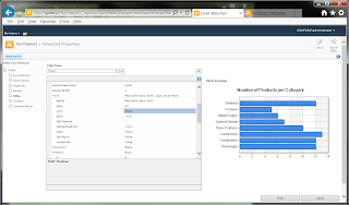
4. As you move the cursor over the chart web part, a dropdown will appear across from the web part title. Click the dropdown, and then point to Advanced Properties.:
   
5. In the Select and Element tree at left, click Series.
6. On the Chart Properties listing, scroll down to the MapArea group.
7. Enter the following URL+keyword string:

   /Northwind2/Lists/Products/AllItems.aspx?FilterField1=Category&FilterValue1=#VALX
   

   
8. Click Finish.
9. Move the cursor over the bars to see the unique URL now configured for each:
   
   Clicking on any bar navigates the browser to the Products list, now filtered by the appropriate category value.  For example, clicking the Seafood bar in the chart, which has a value of 12, navigates the browser to the Products list, which lists 12 seafood items:
   

Optional: Enhance Chart Appearance

1. Launch a browser and then connect to the target page.
2. On the Page ribbon, click Edit Page.
3. As you move the cursor over the chart web part, a dropdown will appear across from the web part title. Click the dropdown, and then point to Advanced Properties.
4. Change Chart Dimensions
1. In the Chart Properties listing, scroll down to the Layout group, and change Width to 500px.
2. Press Enter.  The change is then implemented:
   
   Be sure to press Enter after making each change.  Otherwise, you might lose some changes.
5. Show Interlaced
1. On the Select an Element tree, select Chart Areas.
2. From the Axis Menu, select X axis.
3. In the Chart Properties listing, in the Appearance group, configure as follows (press Enter each time):
1. IsInterlaced: True.
2. InterlacedColor: WhiteSmoke.
3. The changes will be implemented immediately:
   
4. Click Finish.
6. Add Title
1. On the Select an Element tree, select Titles.
2. Click the small + sign just above the top right corner of the Chart Properties list.  This adds a new Title object to the chart, and the Chart Properties listing now displays configurable parameters for this object.
3. In the Appearance group, scrolling down a bit, look for the Text parameter and then set the text to the desired title.
4. Scroll just a bit back up, looking for the Size and Bold parameters, setting these to 12 and True respectively:
   
7. Add Axis Labels
1. On the Select an Element tree, select Chart Areas.
2. From the Axis Menu, select X axis.
3. Scroll down to the Title group.
4. Set the Bold parameter to True.
5. Enter the desired x-axis title into the Title parameter.
6. From the Axis Menu, select Y axis.
7. Scroll down to the Title group.
8. Set the Bold parameter to True.
9. Enter the desired y-axis title into the Title parameter.
10. Now the chart has X and Y axis labels:
    
11. Click Finish.
8. Display each bar in different color
1. On the Select an Element tree, select Series.
2. On the Series Menu, select the desired series (if you have only one series, this will likely display as Default).
3. On the Chart Properties listing, in the Appearance group, scroll down until you see the Palette property.  By default, this will be set to None.
4. Select any other setting available from this dropdown.  The change will be immediate:
   
5. Click Finish.
9. Hide the Data & Appearance and Advanced Properties toolbar
1. For this you will need SharePoint Designer and Design permissions to the site or page.
2. Launch SharePoint Designer 2010.
3. Connect to the site hosting the page containing the chart web part.
4. Checkout the file
5. Detach the file from the layout.
6. Open the page in Advanced edit view.
7. Search for ShowToolbar.
8. Set this parameter to False.
9. Save the file.
10. Check it back in.
10. The final interactive chart:
    

Summary

This posting as shown how to create a no-code drill-down chart in SharePoint 2010.  It has also shown a few ways in which to enhance the chart's appearance.  For additional details on the topics discussed in this posting, see the references below.

References

• Direct
• SharePoint 2010 Northwind Sample Database Site Template
• MSDN Chart Control Keywords
• General
• Built-In Keywords for Series Properties
• Keywords [rs_vsDataVis]
• Using the Chart Web Part with Web Part Data Sources
• Microsoft Chart Control How-to: Add Rich Content Using Keywords

Notes

• The URL defined in Step 4.7 does not include the view ID.  You see this ID when you choose to filter a list by some column value in the list.  You don't need this ID if you are referring to just one list, and this list is located on a different page, such as an application page.  However, if you are building page containing lists, and the charts are referring to those lists, you will need to use the view ID.  Otherwise you will experience this error: One or more field types are not installed properly. Go to the list settings page to delete these fields.
• The method presented here also works for the chart web part in SharePoint 2013.

How to set up Excel Services to use Secure Store Services and an unattended service account

Introduction

BI Services Series

How to implement SharePoint 2010 Access Services

How to setup Secure Store and BCS to access LOB data

How to enable document conversion from Word to HTML in SharePoint 2010

How to set up Excel Services to use Secure Store Services and an unattended service account

This posting walks through the process of configuring SharePoint Server 2010 farm Excel Services to use Secure Store Services and an unattached service account, when presented published Excel 2010 workbooks and workbook objects that connect to external data sources.  Accomplishing this involves the following tasks:

1. Configuring a data access account;
2. Configuring the farm Secure Store target application for the unattended service account;
3. Configuring the farm's Excel Services Global Settings;
4. Configuring a workbook to use the unattended service account when published and connecting to external data sources;
5. Configuring this workbook to publish only user-defined workbook objects to Excel Services; and finally
6. Testing our implementation.

This posting assumes that you already have a workbook created and connected to an external data source; that you have already created a PivotTable; and that you have created a PivotChart in this workbook.  It also assumes that you have configured and started Excel Services on the farm.  This posting employs the AdventureWorks database to present Excel Services, and all development work was performed within an environment hosted on VMware Workstation 7.X.

Preparation

• Identify an Active Directory service account that will serve as the Excel services unattended service account.  This must be a domain account.  It may be an existing farm services account or a new one.
• For this posting, an existing farm services account, contoso\sp_app, will be used.
• Identify the target external data source to which Excel needs access.
• For this posting, the full version of the AdventureWorks database, version 2008R2, will be used.
• Identify a name that you will assign to the Secure Store service application.
• Create or identify a document library on the farm to which you want to publish a workbook.

Step 1: Configure the data access account

1. Launch SQL Server Management Studio.
2. In the console tree, expand Security.
3. Right-click on Logins, and then click New Login.
4. Add the AD account, in this case, contoso\sp_app, and then select Windows Authentication.
5. Select the User Mapping page; select the target database (in this case AdventureWorks Full); and then add the db_datareader role to this account:
   
6. Click OK.
7. This completes Step 1.

Step 2: Configure a new Secure Store target application

1. Connect to Central Administration using a farm administrator account (this is critical).
2. Go: Security > General Security > Configure service accounts.
3. From the Credential Management dropdown, select Service Application Pool - SharePoint Web Services Default:
   
4. Verify that Excel Services Application (Excel Services Application Web Service Application) is listed along with other service applications.
5. Note down the account name associated with this service.  For this posting, the service account is: contoso\sp_app.
6. Click Cancel.
7. Go: Application Management > Manage service applications.  The Manage Service Applications page is displayed:
   
8. Click on Secure Store Service.  The Secure Store Service page is displayed:
   
9. On the Edit ribbon, click the New button.  The Create New Secure Store Target Application Target Application Settings page is displayed.
10. Configure the new Secure Store Target Application.  For this posting, the following configuration was used:
1. Target Application ID: ExcelServicesUnattended.
2. Display Name: ExcelServicesUnattended.
3. Contact Email: Stephan.bren@contoso.com.
4. Target Application Type: Group:
   
5. Click Next. The Create New Secure Store Target Application Add Field page is displayed:
   
6. Leave all settings default, and then click Next.  The Create New Secure Store Target Application Specify the membership settings page is displayed.
7. Enter user accounts who for administration and the unattended account that will be mapped to this secure store application:
   
8. Click OK.  The browser is returned to the Secure Store Service Target Application page, now displaying the new Target Application name:
   
9. Check the new target application item listed, and then, on the Edit ribbon, click the Set Credentials button.  The Set Credentials for Secure Store Target Application (Group) dialog appears.
10. In this dialog, enter the same domain account and password that was used in Step 1:
    
    For this posting, these accounts are the same, but they need not be.
11. Click OK.
11. This completes Step 2.

Step 3: Configure Excel Services Global Settings

1. From Central Administration, go: Application Management > Manage Service Applications:
   
2. Click Excel Services.
3. Click Global Settings, and then scroll down to the External Data section.
4. In the Application ID field, enter the same name that was assigned to the Target Application ID, back in step 2.  For this posting, the Target Application ID is ExcelServicesUnattended:
   
5. Click OK.
6. This completes Step 3.

Step 4: Configure the workbook to use the unattended service account

1. Open the Excel 2010 workbook that you want to publish and that is connected to an external data source:
   
2. On the Data ribbon, click the Connections button.  The Workbook Connections dialog appears:
   
3. Click the Properties button.  The Connection Properties dialog appears:
   
4. Check off all of the options that you see, and then select the Definitions tab:
   
• The Command Text and Command Type are custom.  For additional information on these, see the Notes section, below.  The SQL that you see there is the following:
  
5. Click the Authentication Settings button.  The Excel Services Authentication Settings dialog appears.
6. Select None:
   
7. Click OK.  The Excel Services Authentication Settings dialog closes.
8. Click OK again.  The Connection Properties dialog closes.
9. Click OK one more time.  The Workbook Connections dialog closes.
10. This completes this Step 4.

Step 5: Configure Workbook objects to be published

1. Select the PivotChart that you want to be published.
2. On the Layout ribbon, click the Properties button.  The small Chart Name box appears just below the button.
3. Enter a defined name for this chart object.  For this posting, the defined name for the chart will be MyChart:
   
   Incidentally, this particular chart already has filters applied: the date range has between filtered to between 7/3/2005 and 7/30/2005. This filtering is not fixed and can be modified even after publication to the farm.  We'll see how later.
4. Press the Enter key.  The little dialog closes, and now when you select the chart, the defined name for the chart will appear in the Name box.
5. Select the File tab.  The File options are displayed.
6. On the File tab, select the Save & Send option, and then select Save to SharePoint:
   
   .
7. Click the Publish Options button.  The Publish Options dialog is displayed.
8. On the Show tab, from the dropdown, select items in the Workbook; then check the MyChart and PivotTable2 objects listed below:
   
9. Click OK.  The dialog closes.
10. This completes Step 5. All configuration has now been completed and it remains to test the implementation.

Step 6: Perform a test publication of the workbook

1. Double-click where it states, Browse for a location.  A Save As dialog appears:.
2. Enter the URL to the document library identified or created at the beginning of this posting.  For this posting, the URL is:

   http://spdev12/AdventureWorks/Workbooks/

   
3. Press the Enter key.  After a few moments, the target SharePoint document library will be shown on the Save As dialog:
   
4. Press the Enter key again.  The dialog closes.  After a few moments, a new browser instance is launched that displays the published workbook chart:
   
   Note that it displays the same filtered view that was previously configured in the local workbook copy itself.
5. To change the filter and interact with the chart, look for the View dropdown, in the upper right corner, and then select PivotTable2 from this dropdown.  The view changes to display the PivotChart's data:
   
6. Change the filter settings as desired, and then return to the PivotChart (in this case MyChart) object to see the affect:
   
7. This completes Step 6.

Optional: Display the PivotChart in a Dashboard

1. Navigate to the target site dashboard page.
2. On the Page ribbon, click the Edit Page button.  The page enters edit mode:
   
3. Click where it states, Add a Web Part, in the web part zone to which you want to add the image.  The Browse ribbon gets the focus and displays tools for finding and selecting a web part.
4. In the Categories panel, click Business Data, and then in the Web Parts panel, select Excel Web Access:
   
5. Click the Add button.  The Browse button is updated, and the page body is updated to display the added web part in edit mode:
   
6. Click the link, Click here to open the tool pane.  The Excel Web Access toolpane is displayed:
   
7. Click the ellipsis box next to the Workbook field.  The Select an Asset -- Webpage Dialog appears:
   
8. In this dialog, navigate to the location of the published workbook.  For this posting, the workbook is located in the Workbooks document library in the AdventureWorks site:
   
9. Click OK.  A progress indicator appears for a few moments, and then the dialog closes, with the workbook path now displayed in the Workbook field on the Excel Web Access toolpane:
   
10. Click OK.  The toolpane closes, and the PivotChart is now displayed in the web part:
    
11. To expand the web part so as to eliminate the scroll bars, from the title toolbar, just above the web part, select the Edit Web Part option.  The Excel Web Access toolpane opens.
12. Scroll down to the Appearance section, and expand this section.
1. Select Yes for both the Height and Width fields;
2. enter 475 for height and
3. enter 580 for width; and then
4. select None from the Chrome Type dropdown:
   
13. Click OK, and then on the Page ribbon, click the Stop Editing button; then select the Browse tab.  The PivotTable is displayed as it would appear to any user:
    
14. To remove the PivotChart toolbar (File, Data, Find, etc), go back to the Toolpane, and then select None from the Type of Toolbar dropdown in the Title  Bar section.  You might also want to uncheck All Workbook Interactivity in the Navigation and Interactivity section.  After making these changes, the PivotChart displays as a simple image:
    
15. This completes the Optional step.

Summary

This posting has presented the steps necessary for how to setup SharePoint Server 2010 Excel Services to use Secure Store Services and the unattended service account when presenting Excel workbook objects, such as PivotCharts and tables.  For additional detail on any topic discussed here, see the references below.

References

• TechNet SQL Server 2008 R2
• The data connection uses Windows Authentication and user credentials could not be delegated. The following connections failed to refresh: PowerPivot Data
• This workbook contains one or more queries that refresh external data
• The data connection uses Windows Authentication and user credentials could not be delegated. The following connections failed to refresh: PowerPivot Data
• CodePlex SQL Server Product Samples
• AdventureWorks2008R2-Full Database Backup
• TechNet SharePoint 2010
• Configure Excel Services data refresh by using the unattended service account (SharePoint Server 2010)
• Microsoft Office Excel 2010
• Refresh connected (imported) data
• View a named item in Excel Services
• Excel Web Access Web Part custom properties
• Using Excel Services to share pieces and parts of Excel workbooks
• Using charts and PivotChart reports in a workbook in the browser
• Blogs
• SharePoint 2010: Creating dashboards and Charts for SharePoint Lists using PerformancePoint and Excel Services from Start to Finish
• Excel Chart Updating with Pivot table

Notes

• Step 4: Excel Services Authentication Settings dialog: Selecting None here is essential.  By selecting None, Excel Services uses the unattended service account identity to establish the connection to the external data source.
• Step 5: Publish Options dialog: Selecting specific items will impact the user's online experience when viewing the published workbook later on.  Selection of the appropriate objects here is important: if you want to only present the PivotChart, then only select the chart object and nothing else. If you want to publish the chart and also enable users to interact with the chart, you must select the chart object and the its data source, which in this case is the PivotTable2 object.  The reason being that published PivotCharts cannot be made directly interactive.  The way to work around this is to provide access to the underlying chart data, and the filter methods associated with that data.  We'll see this later once the workbook objects are published.
• Optional: Select an Asset -- Webpage Dialog: note that you can navigate to any asset (workbook) within the site collection - not just to assets within the current site.

References

Sunday, October 27, 2013